pacman::p_load(tidyverse,ggridges,ggrepel,ggthemes,ggstatsplot,ggsignif,
               hrbrthemes,patchwork,dplyr, gifski, gapminder,plotly,
gganimate,ggiraph,magick,highcharter,knitr,naniar,DT,imputeTS,ggHoriPlot,stars,terra,gstat,RColorBrewer)Take-home exercise 4 Visual Analytics
1 Overview
For this Take Home Exercise, there are several task needs to be done to create the Shiny application.
To evaluate and determine the necessary R packages needed for your Shiny application are supported in R CRAN,
To prepare and test the specific R codes can be run and returned the correct output as expected,
To determine the parameters and outputs that will be exposed on the Shiny applications, and
To select the appropriate Shiny UI components for exposing the parameters determine above.
This submission includes the prototype report for the group project, which will includes:
the data preparation process,
the selection of data visualization techniques used,
and the data visualization design and interactivity principles and best practices implemented.
Based on the discussion with team member i will be focusing on the Exploratory Data Analysis & Confirmatory Data Analysis, and the UI design for our Shiny app.
2 Project Information
The purpose of this project is to create a Shiny app with user-friendly interface and functions, and also create a website for user to discover the historical Weather changes in Singapore.
3 Get Started (Load R Packages)
4 . Data Preparation
import the merged data of all the stations across 10 years (2014-2023)
rfdata <- read.csv('data/merged_data.csv')Import the data that includes the latitude and longitude of the weather stations in Singapore.
rfstation <- read.csv('data/RainfallStation.csv')

rfstation <- rfstation %>%
  rename(Station = Station.Code)
Join the latitude and longitude to the rfdata, so that in the analysis part we can map the geospatial analysis.
raw_weather_data <- rfdata  %>%
  left_join(rfstation, by = "Station")
This dataset was retrieved from the Meteorological Service Singapore site, and had some basic pre-processing steps performed in python due to the large amount of files:
Combine all downloaded CSV files into one dataframe.
Add the latitude and longitude of each station to the data frame.
4.1 Check structure with glimpse()
glimpse(raw_weather_data)Rows: 204,464
Columns: 15
$ Station <chr> "Paya Lebar", "Paya Lebar", "Paya Lebar"…
$ Year <int> 2014, 2014, 2014, 2014, 2014, 2014, 2014…
$ Month <int> 1, 1, 1, 1, 1, 1, 1, 1, 1, 1, 1, 1, 1, 1…
$ Day <int> 1, 2, 3, 4, 5, 6, 7, 8, 9, 10, 11, 12, 1…
$ Daily.Rainfall.Total..mm. <chr> "0", "0", "2.2", "0.6", "10.5", "31.2", …
$ Highest.30.min.Rainfall..mm. <chr> "�", "�", "�", "�", "�", "�", "�", "�", …
$ Highest.60.min.Rainfall..mm. <chr> "�", "�", "�", "�", "�", "�", "�", "�", …
$ Highest.120.min.Rainfall..mm. <chr> "�", "�", "�", "�", "�", "�", "�", "�", …
$ Mean.Temperature...C. <chr> "�", "�", "�", "�", "�", "�", "�", "�", …
$ Maximum.Temperature...C. <chr> "29.5", "31.7", "31.1", "32.3", "27", "2…
$ Minimum.Temperature...C. <chr> "24.8", "25", "25.1", "23.7", "23.8", "2…
$ Mean.Wind.Speed..km.h. <chr> "15.8", "16.5", "14.9", "8.9", "11.9", "…
$ Max.Wind.Speed..km.h. <chr> "35.3", "37.1", "33.5", "35.3", "33.5", …
$ Latitude <dbl> 1.3524, 1.3524, 1.3524, 1.3524, 1.3524, …
$ Longitude <dbl> 103.9007, 103.9007, 103.9007, 103.9007, …There are 204464 rows, and 15 columns in the dataset. We see that there are missing values shown as ‘?’ in the dataset. In the next few steps, we will drop specific columns and rows based on the project focus.
4.2 Drop unused columns
We will not be using all 15 columns for this project. The following columns will be dropped:
Highest 30 Min Rainfall (mm)Highest 60 Min Rainfall (mm)Highest 1200 Min Rainfall (mm)Mean Wind Speed (km/h)Max Wind Speed (km/h)
raw_weather_data <- raw_weather_data %>%
  select(-c(`Highest.30.min.Rainfall..mm.`,
            `Highest.60.min.Rainfall..mm.`,
            `Highest.120.min.Rainfall..mm.`,
            `Mean.Wind.Speed..km.h.`,
            `Max.Wind.Speed..km.h.`))
4.3 Remove rows for specific Stations
The Meteorological Service Singapore also provides a file, Station Records that has some information on the availability of data for each station. After examining the station records file, we found that 41 stations had missing information for some variables. We will hence drop rows for these stations.
# Drop rows of 41 stations
# Define the station names to remove
stations_to_remove <- c("Macritchie Reservoir", "Lower Peirce Reservoir", "Pasir Ris (West)", "Kampong Bahru", "Jurong Pier", "Ulu Pandan", "Serangoon", "Jurong (East)", "Mandai", "Upper Thomson", "Buangkok", "Boon Lay (West)", "Bukit Panjang", "Kranji Reservoir", "Tanjong Pagar", "Admiralty West", "Queenstown", "Tanjong Katong", "Chai Chee", "Upper Peirce Reservoir", "Kent Ridge", "Somerset (Road)", "Punggol", "Tuas West", "Simei", "Toa Payoh", "Tuas", "Bukit Timah", "Yishun", "Buona Vista", "Pasir Ris (Central)", "Jurong (North)", "Choa Chu Kang (West)", "Serangoon North", "Lim Chu Kang", "Marine Parade", "Choa Chu Kang (Central)", "Dhoby Ghaut", "Nicoll Highway", "Botanic Garden", "Whampoa")

# Remove rows with the specified station names
raw_weather_data <- raw_weather_data[!raw_weather_data$Station %in% stations_to_remove, ]

# Print the number of stations left
print(sprintf(" %d stations removed. %d stations left.", length(stations_to_remove), n_distinct(raw_weather_data$Station)))
[1] " 41 stations removed. 22 stations left."4.4 Check for duplicates
# Identify duplicates
duplicates <- raw_weather_data[duplicated(raw_weather_data[c("Station", "Year", "Month", "Day")]) | duplicated(raw_weather_data[c("Station", "Year", "Month", "Day")], fromLast = TRUE), ]

# Check if 'duplicates' dataframe is empty
if (nrow(duplicates) == 0) {
  print("The combination of Station Name, Year, Month, and Day is unique.")
} else {
  print("There are duplicates in the combination of Station Name, Year, Month, and Day. Showing duplicated rows:")
  print(duplicates)
}
[1] "There are duplicates in the combination of Station Name, Year, Month, and Day. Showing duplicated rows:"
Station Year Month Day Daily.Rainfall.Total..mm.
13381 Semakau Island NA NA NA -
13382 Semakau Island NA NA NA -
13383 Semakau Island NA NA NA -
13384 Semakau Island NA NA NA -
13385 Semakau Island NA NA NA -
13386 Semakau Island NA NA NA -
13387 Semakau Island NA NA NA -
13388 Semakau Island NA NA NA -
13389 Semakau Island NA NA NA -
13390 Semakau Island NA NA NA -
13391 Semakau Island NA NA NA -
13392 Semakau Island NA NA NA -
13393 Semakau Island NA NA NA -
13394 Semakau Island NA NA NA -
13395 Semakau Island NA NA NA -
13396 Semakau Island NA NA NA -
13397 Semakau Island NA NA NA -
13398 Semakau Island NA NA NA -
13399 Semakau Island NA NA NA -
13400 Semakau Island NA NA NA -
13401 Semakau Island NA NA NA -
13402 Semakau Island NA NA NA -
13403 Semakau Island NA NA NA -
13404 Semakau Island NA NA NA -
13405 Semakau Island NA NA NA -
13406 Semakau Island NA NA NA -
13407 Semakau Island NA NA NA -
13408 Semakau Island NA NA NA -
13409 Semakau Island NA NA NA -
13410 Semakau Island NA NA NA -
13411 Semakau Island NA NA NA -
13412 Semakau Island NA NA NA -
13413 Semakau Island NA NA NA -
13414 Semakau Island NA NA NA -
13415 Semakau Island NA NA NA -
13416 Semakau Island NA NA NA -
13417 Semakau Island NA NA NA -
13418 Semakau Island NA NA NA -
13419 Semakau Island NA NA NA -
13420 Semakau Island NA NA NA -
13421 Semakau Island NA NA NA -
13422 Semakau Island NA NA NA -
13423 Semakau Island NA NA NA -
13424 Semakau Island NA NA NA -
13425 Semakau Island NA NA NA -
13426 Semakau Island NA NA NA -
13427 Semakau Island NA NA NA -
13428 Semakau Island NA NA NA -
13429 Semakau Island NA NA NA -
13430 Semakau Island NA NA NA -
13431 Semakau Island NA NA NA -
13432 Semakau Island NA NA NA -
13433 Semakau Island NA NA NA -
13434 Semakau Island NA NA NA -
13435 Semakau Island NA NA NA -
13436 Semakau Island NA NA NA -
13437 Semakau Island NA NA NA -
13438 Semakau Island NA NA NA -
13439 Semakau Island NA NA NA -
13440 Semakau Island NA NA NA -
13441 Semakau Island NA NA NA -
14084 Semakau Island NA NA NA -
14085 Semakau Island NA NA NA -
14086 Semakau Island NA NA NA -
14087 Semakau Island NA NA NA -
14088 Semakau Island NA NA NA -
183829 Boon Lay (East) NA NA NA -
183830 Boon Lay (East) NA NA NA -
183831 Boon Lay (East) NA NA NA -
183832 Boon Lay (East) NA NA NA -
183833 Boon Lay (East) NA NA NA -
183834 Boon Lay (East) NA NA NA -
183835 Boon Lay (East) NA NA NA -
183836 Boon Lay (East) NA NA NA -
183837 Boon Lay (East) NA NA NA -
183838 Boon Lay (East) NA NA NA -
183839 Boon Lay (East) NA NA NA -
183840 Boon Lay (East) NA NA NA -
183841 Boon Lay (East) NA NA NA -
183842 Boon Lay (East) NA NA NA -
183843 Boon Lay (East) NA NA NA -
183844 Boon Lay (East) NA NA NA -
183845 Boon Lay (East) NA NA NA -
183846 Boon Lay (East) NA NA NA -
183847 Boon Lay (East) NA NA NA -
183848 Boon Lay (East) NA NA NA -
183849 Boon Lay (East) NA NA NA -
183850 Boon Lay (East) NA NA NA -
183851 Boon Lay (East) NA NA NA -
183852 Boon Lay (East) NA NA NA -
183853 Boon Lay (East) NA NA NA -
183854 Boon Lay (East) NA NA NA -
183855 Boon Lay (East) NA NA NA -
183856 Boon Lay (East) NA NA NA -
183857 Boon Lay (East) NA NA NA -
183858 Boon Lay (East) NA NA NA -
191071 Boon Lay (East) NA NA NA -
191072 Boon Lay (East) NA NA NA -
191073 Boon Lay (East) NA NA NA -
191074 Boon Lay (East) NA NA NA -
191075 Boon Lay (East) NA NA NA -
191076 Boon Lay (East) NA NA NA -
191077 Boon Lay (East) NA NA NA -
191078 Boon Lay (East) NA NA NA -
191079 Boon Lay (East) NA NA NA -
191080 Boon Lay (East) NA NA NA -
191081 Boon Lay (East) NA NA NA -
191082 Boon Lay (East) NA NA NA -
191083 Boon Lay (East) NA NA NA -
191084 Boon Lay (East) NA NA NA -
191085 Boon Lay (East) NA NA NA -
191086 Boon Lay (East) NA NA NA -
191087 Boon Lay (East) NA NA NA -
191088 Boon Lay (East) NA NA NA -
191089 Boon Lay (East) NA NA NA -
191090 Boon Lay (East) NA NA NA -
191091 Boon Lay (East) NA NA NA -
191092 Boon Lay (East) NA NA NA -
191093 Boon Lay (East) NA NA NA -
191094 Boon Lay (East) NA NA NA -
191095 Boon Lay (East) NA NA NA -
191096 Boon Lay (East) NA NA NA -
191097 Boon Lay (East) NA NA NA -
191098 Boon Lay (East) NA NA NA -
191099 Boon Lay (East) NA NA NA -
191100 Boon Lay (East) NA NA NA -
191101 Boon Lay (East) NA NA NA -
Mean.Temperature...C. Maximum.Temperature...C. Minimum.Temperature...C.
13381 - - -
13382 - - -
13383 - - -
13384 - - -
13385 - - -
13386 - - -
13387 - - -
13388 - - -
13389 - - -
13390 - - -
13391 - - -
13392 - - -
13393 - - -
13394 - - -
13395 - - -
13396 - - -
13397 - - -
13398 - - -
13399 - - -
13400 - - -
13401 - - -
13402 - - -
13403 - - -
13404 - - -
13405 - - -
13406 - - -
13407 - - -
13408 - - -
13409 - - -
13410 - - -
13411 - - -
13412 - - -
13413 - - -
13414 - - -
13415 - - -
13416 - - -
13417 - - -
13418 - - -
13419 - - -
13420 - - -
13421 - - -
13422 - - -
13423 - - -
13424 - - -
13425 - - -
13426 - - -
13427 - - -
13428 - - -
13429 - - -
13430 - - -
13431 - - -
13432 - - -
13433 - - -
13434 - - -
13435 - - -
13436 - - -
13437 - - -
13438 - - -
13439 - - -
13440 - - -
13441 - - -
14084 - - -
14085 - - -
14086 - - -
14087 - - -
14088 - - -
183829 - - -
183830 - - -
183831 - - -
183832 - - -
183833 - - -
183834 - - -
183835 - - -
183836 - - -
183837 - - -
183838 - - -
183839 - - -
183840 - - -
183841 - - -
183842 - - -
183843 - - -
183844 - - -
183845 - - -
183846 - - -
183847 - - -
183848 - - -
183849 - - -
183850 - - -
183851 - - -
183852 - - -
183853 - - -
183854 - - -
183855 - - -
183856 - - -
183857 - - -
183858 - - -
191071 - - -
191072 - - -
191073 - - -
191074 - - -
191075 - - -
191076 - - -
191077 - - -
191078 - - -
191079 - - -
191080 - - -
191081 - - -
191082 - - -
191083 - - -
191084 - - -
191085 - - -
191086 - - -
191087 - - -
191088 - - -
191089 - - -
191090 - - -
191091 - - -
191092 - - -
191093 - - -
191094 - - -
191095 - - -
191096 - - -
191097 - - -
191098 - - -
191099 - - -
191100 - - -
191101 - - -
Latitude Longitude
13381 1.1890 103.7680
13382 1.1890 103.7680
13383 1.1890 103.7680
13384 1.1890 103.7680
13385 1.1890 103.7680
13386 1.1890 103.7680
13387 1.1890 103.7680
13388 1.1890 103.7680
13389 1.1890 103.7680
13390 1.1890 103.7680
13391 1.1890 103.7680
13392 1.1890 103.7680
13393 1.1890 103.7680
13394 1.1890 103.7680
13395 1.1890 103.7680
13396 1.1890 103.7680
13397 1.1890 103.7680
13398 1.1890 103.7680
13399 1.1890 103.7680
13400 1.1890 103.7680
13401 1.1890 103.7680
13402 1.1890 103.7680
13403 1.1890 103.7680
13404 1.1890 103.7680
13405 1.1890 103.7680
13406 1.1890 103.7680
13407 1.1890 103.7680
13408 1.1890 103.7680
13409 1.1890 103.7680
13410 1.1890 103.7680
13411 1.1890 103.7680
13412 1.1890 103.7680
13413 1.1890 103.7680
13414 1.1890 103.7680
13415 1.1890 103.7680
13416 1.1890 103.7680
13417 1.1890 103.7680
13418 1.1890 103.7680
13419 1.1890 103.7680
13420 1.1890 103.7680
13421 1.1890 103.7680
13422 1.1890 103.7680
13423 1.1890 103.7680
13424 1.1890 103.7680
13425 1.1890 103.7680
13426 1.1890 103.7680
13427 1.1890 103.7680
13428 1.1890 103.7680
13429 1.1890 103.7680
13430 1.1890 103.7680
13431 1.1890 103.7680
13432 1.1890 103.7680
13433 1.1890 103.7680
13434 1.1890 103.7680
13435 1.1890 103.7680
13436 1.1890 103.7680
13437 1.1890 103.7680
13438 1.1890 103.7680
13439 1.1890 103.7680
13440 1.1890 103.7680
13441 1.1890 103.7680
14084 1.1890 103.7680
14085 1.1890 103.7680
14086 1.1890 103.7680
14087 1.1890 103.7680
14088 1.1890 103.7680
183829 1.3302 103.7205
183830 1.3302 103.7205
183831 1.3302 103.7205
183832 1.3302 103.7205
183833 1.3302 103.7205
183834 1.3302 103.7205
183835 1.3302 103.7205
183836 1.3302 103.7205
183837 1.3302 103.7205
183838 1.3302 103.7205
183839 1.3302 103.7205
183840 1.3302 103.7205
183841 1.3302 103.7205
183842 1.3302 103.7205
183843 1.3302 103.7205
183844 1.3302 103.7205
183845 1.3302 103.7205
183846 1.3302 103.7205
183847 1.3302 103.7205
183848 1.3302 103.7205
183849 1.3302 103.7205
183850 1.3302 103.7205
183851 1.3302 103.7205
183852 1.3302 103.7205
183853 1.3302 103.7205
183854 1.3302 103.7205
183855 1.3302 103.7205
183856 1.3302 103.7205
183857 1.3302 103.7205
183858 1.3302 103.7205
191071 1.3302 103.7205
191072 1.3302 103.7205
191073 1.3302 103.7205
191074 1.3302 103.7205
191075 1.3302 103.7205
191076 1.3302 103.7205
191077 1.3302 103.7205
191078 1.3302 103.7205
191079 1.3302 103.7205
191080 1.3302 103.7205
191081 1.3302 103.7205
191082 1.3302 103.7205
191083 1.3302 103.7205
191084 1.3302 103.7205
191085 1.3302 103.7205
191086 1.3302 103.7205
191087 1.3302 103.7205
191088 1.3302 103.7205
191089 1.3302 103.7205
191090 1.3302 103.7205
191091 1.3302 103.7205
191092 1.3302 103.7205
191093 1.3302 103.7205
191094 1.3302 103.7205
191095 1.3302 103.7205
191096 1.3302 103.7205
191097 1.3302 103.7205
191098 1.3302 103.7205
191099 1.3302 103.7205
191100 1.3302 103.7205
191101 1.3302 103.72054.5 Check and handle missing values
4.5.1 First check for missing values
Missing values in this dataset can be represented by:
\u0097NA-
We first replace these values with actual NA values:
raw_weather_data <- raw_weather_data %>%
  mutate(across(where(is.character), ~na_if(.x, "\u0097"))) %>%
  mutate(across(where(is.character), ~na_if(.x, "NA"))) %>%
  mutate(across(where(is.character), ~na_if(.x, "-")))
Next, we visualize the missing values in the dataset:
# For a simple missing data plot
gg_miss_var(raw_weather_data)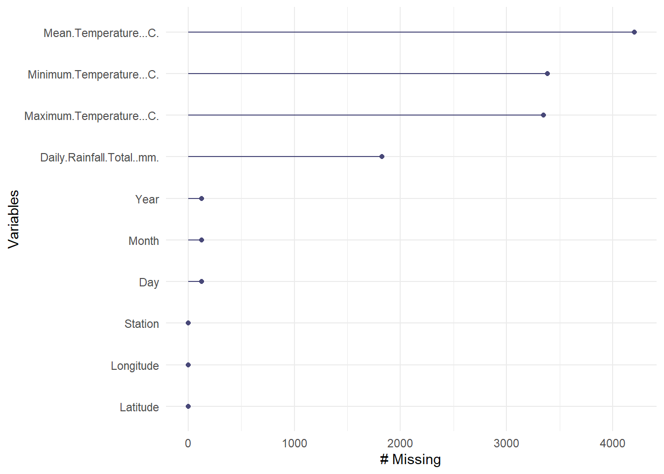
We can see there is quite a number of missing data in the Mean Temperature, Minimum Temperature, Maximum Temperature and Daily Rainfall Total. We will take steps to handle the missing data.
4.5.2 Remove Stations with significant missing data
We have identified two checks to make:
Check which stations have no recorded data for entire months.
Check which stations have more than 7 consecutive days of missing data
For both these checks, we will remove the entire station from the dataset as it would not be practical to impute such large amounts of missing values.
4.5.3 Identify and remove Stations with no recorded data for entire months
Some stations have no recorded data for entire months, as summarised in the table below:
# Create complete combination of Station, Year, and Month
all_combinations <- expand.grid(
  Station = unique(raw_weather_data$Station),
  Year = 2021:2023,
  Month = 1:12
)

# Left join this with the original weather data to identify missing entries
missing_months <- all_combinations %>%
  left_join(raw_weather_data, by = c("Station", "Year", "Month")) %>%
  # Use is.na() to check for rows that didn't have a match in the original data
  filter(is.na(Day)) %>%
  # Select only the relevant columns for the final output
  select(Station, Year, Month)

# Create a summary table that lists out the missing months
missing_months_summary <- missing_months %>%
  group_by(Station, Year) %>%
  summarise(MissingMonths = toString(sort(unique(Month))), .groups = 'drop')

kable(missing_months_summary)| Station | Year | MissingMonths |
|---|---|---|
| Boon Lay (East) | 2021 | 1, 2, 3, 4, 5, 6, 7, 8, 9, 10, 11, 12 |
| Boon Lay (East) | 2022 | 1, 2, 3, 4, 5, 6, 7, 8, 9, 10, 11, 12 |
| Boon Lay (East) | 2023 | 1, 2, 3, 4, 5, 6, 7, 8, 9, 10, 11, 12 |
| Khatib | 2022 | 1, 2, 3, 4, 5, 6, 7, 8, 9, 10, 11, 12 |
| Khatib | 2023 | 1, 2, 3, 4, 5, 6, 7, 8, 9, 10, 11, 12 |
We hence drop these stations from our dataset:
raw_weather_data <- anti_join(raw_weather_data, missing_months, by = "Station")

print(sprintf("The folowing %d stations were dropped: %s", n_distinct(missing_months$Station), paste(unique(missing_months$Station), collapse = ", ")))
[1] "The folowing 2 stations were dropped: Boon Lay (East), Khatib"print(sprintf("There are %d stations left: ", n_distinct(raw_weather_data$Station)))[1] "There are 20 stations left: "kable(unique(raw_weather_data$Station),
row.names = TRUE,
col.names = "Station",
caption = "List of Remaining Stations")| Station | |
|---|---|
| 1 | Paya Lebar |
| 2 | Semakau Island |
| 3 | Admiralty |
| 4 | Pulau Ubin |
| 5 | East Coast Parkway |
| 6 | Marina Barrage |
| 7 | Ang Mo Kio |
| 8 | Newton |
| 9 | Jurong Island |
| 10 | Tuas South |
| 11 | Pasir Panjang |
| 12 | Choa Chu Kang (South) |
| 13 | Tengah |
| 14 | Changi |
| 15 | Seletar |
| 16 | Tai Seng |
| 17 | Jurong (West) |
| 18 | Clementi |
| 19 | Sentosa Island |
| 20 | Sembawang |
4.5.4 Identify and remove Stations with excessive missing values
If there are any missing values, we can try to impute these missing values. However, if there are 7 or more consecutive values missing, we will remove these stations first.
# Define a helper function to count the number of 7 or more consecutive NAs
count_seven_consecutive_NAs <- function(x) {
  na_runs <- rle(is.na(x))
  total_consecutive_NAs <- sum(na_runs$lengths[na_runs$values & na_runs$lengths >= 7])
  return(total_consecutive_NAs)
}

# Apply the helper function to each relevant column within grouped data
weather_summary <- raw_weather_data %>%
  group_by(Station, Year, Month) %>%
  summarise(across(-Day, ~ count_seven_consecutive_NAs(.x), .names = "count_consec_NAs_{.col}"), .groups = "drop")

# Filter to keep only rows where there is at least one column with 7 or more consecutive missing values
weather_summary_with_consecutive_NAs <- weather_summary %>%
  filter(if_any(starts_with("count_consec_NAs_"), ~ . > 0))

# View the result
print(sprintf("There are %d stations with 7 or more consecutive missing values.", n_distinct(weather_summary_with_consecutive_NAs$Station)))
[1] "There are 13 stations with 7 or more consecutive missing values."# kable(weather_summary_with_consecutive_NAs)
datatable(weather_summary_with_consecutive_NAs,
class= "compact",
rownames = FALSE,
width="100%",
options = list(pageLength = 10, scrollX=T),
caption = 'Details of stations with >=7 missing values')We hence drop these stations from our dataset:
raw_weather_data <- anti_join(raw_weather_data, weather_summary_with_consecutive_NAs, by = "Station")

print(sprintf("The folowing %d stations were dropped: %s", n_distinct(weather_summary_with_consecutive_NAs$Station), paste(unique(weather_summary_with_consecutive_NAs$Station), collapse = ", ")))
[1] "The folowing 13 stations were dropped: Admiralty, Ang Mo Kio, Clementi, Jurong Island, Marina Barrage, Paya Lebar, Pulau Ubin, Seletar, Semakau Island, Sembawang, Sentosa Island, Tengah, Tuas South"print(sprintf("There are %d stations left: ", n_distinct(raw_weather_data$Station)))[1] "There are 7 stations left: "kable(unique(raw_weather_data$Station),
row.names = TRUE,
col.names = "Station",
caption = "List of Remaining Stations")| Station | |
|---|---|
| 1 | East Coast Parkway |
| 2 | Newton |
| 3 | Pasir Panjang |
| 4 | Choa Chu Kang (South) |
| 5 | Changi |
| 6 | Tai Seng |
| 7 | Jurong (West) |
4.5.5 Second check for missing values
From the check below we see there are still missing values in our data. We will impute these values in the next step.
# For a simple missing data plot
gg_miss_var(raw_weather_data)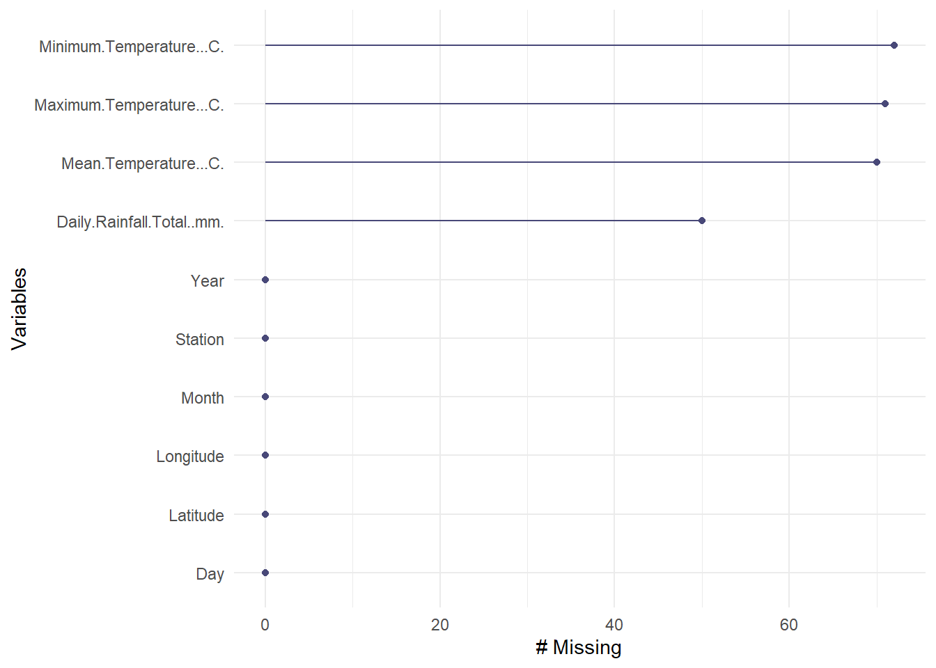
We can see that there is still a few missing values from the selected stations.
4.6 Impute missing values
To handle the missing values for the remaining Stations, we will impute missing values using simple moving average from imputeTS package.
raw_weather_data <- raw_weather_data %>%
  mutate(Date = as.Date(paste(Year, Month, Day, sep = "-"))) %>%
  relocate(Date, .after = 1)
# Define the weather variables to loop through
weather_variables <- c("Daily.Rainfall.Total..mm.", "Mean.Temperature...C.", "Maximum.Temperature...C.", "Minimum.Temperature...C.")
# Ensure raw_weather_data is correctly copied to a new data frame for imputation
weather_data_imputed <- raw_weather_data
# Loop through each weather variable to impute missing values
for(variable in weather_variables) {
# Convert variable to numeric, ensuring that the conversion warnings are handled if necessary
weather_data_imputed[[variable]] <- as.numeric(as.character(weather_data_imputed[[variable]]))
# Impute missing values using a moving average
weather_data_imputed <- weather_data_imputed %>%
group_by(Station) %>%
arrange(Station, Date) %>%
mutate("{variable}" := round(na_ma(.data[[variable]], k = 7, weighting = "simple"), 1)) %>%
ungroup()
}4.7 Add specific columns to data [NEW]
These columns are added as they may be used in plots later.
weather_data_imputed <- weather_data_imputed %>%
  mutate(Date_mine = make_date(2023, month(Date), day(Date)),
         Month_Name = factor(months(Date), levels = month.name),
         Week = isoweek(Date),
         Weekday = wday(Date)
  )
4.8 Summary of cleaned data
Details of stations and time period of data
time_period_start <- min(weather_data_imputed$Date)
time_period_end <- max(weather_data_imputed$Date)
cat("\nThe time period of the dataset is from", format(time_period_start, "%Y-%m-%d"),"to", format(time_period_end, "%Y-%m-%d"), "\n")
The time period of the dataset is from 2014-01-01 to 2024-01-31 but i only want to keep until 2023, exclude record in 2024
weather_data_imputed <- subset(weather_data_imputed, Date <= as.Date("2023-12-31"))

time_period_start <- min(weather_data_imputed$Date)
time_period_end <- max(weather_data_imputed$Date)
cat("\nThe time period of the dataset is from", format(time_period_start, "%Y-%m-%d"),"to", format(time_period_end, "%Y-%m-%d"), "\n")
The time period of the dataset is from 2014-01-01 to 2023-12-31 And also to ease further analysis, convert year, month, day to factor data type:
weather_data_imputed <- weather_data_imputed %>%
  mutate_at(vars(Year,Month,Day),as.factor)

glimpse(weather_data_imputed)
Rows: 25,258
Columns: 15
$ Station <chr> "Changi", "Changi", "Changi", "Changi", "Cha…
$ Date <date> 2014-01-01, 2014-01-02, 2014-01-03, 2014-01…
$ Year <fct> 2014, 2014, 2014, 2014, 2014, 2014, 2014, 20…
$ Month <fct> 1, 1, 1, 1, 1, 1, 1, 1, 1, 1, 1, 1, 1, 1, 1,…
$ Day <fct> 1, 2, 3, 4, 5, 6, 7, 8, 9, 10, 11, 12, 13, 1…
$ Daily.Rainfall.Total..mm. <dbl> 0.0, 0.0, 0.0, 0.0, 18.4, 31.2, 0.0, 0.0, 2.…
$ Mean.Temperature...C. <dbl> 26.7, 27.4, 27.1, 27.1, 24.8, 25.3, 26.7, 27…
$ Maximum.Temperature...C. <dbl> 29.0, 30.9, 30.4, 31.1, 26.4, 27.1, 30.7, 31…
$ Minimum.Temperature...C. <dbl> 24.9, 25.0, 24.9, 24.9, 23.3, 23.9, 24.3, 24…
$ Latitude <dbl> 1.3678, 1.3678, 1.3678, 1.3678, 1.3678, 1.36…
$ Longitude <dbl> 103.9826, 103.9826, 103.9826, 103.9826, 103.…
$ Date_mine <date> 2023-01-01, 2023-01-02, 2023-01-03, 2023-01…
$ Month_Name <fct> January, January, January, January, January,…
$ Week <dbl> 1, 1, 1, 1, 1, 2, 2, 2, 2, 2, 2, 2, 3, 3, 3,…
$ Weekday <dbl> 4, 5, 6, 7, 1, 2, 3, 4, 5, 6, 7, 1, 2, 3, 4,…kable(unique(weather_data_imputed$Station),
row.names = TRUE,
col.names = "Station",
caption = "List of Stations")| Station | |
|---|---|
| 1 | Changi |
| 2 | Choa Chu Kang (South) |
| 3 | East Coast Parkway |
| 4 | Jurong (West) |
| 5 | Newton |
| 6 | Pasir Panjang |
| 7 | Tai Seng |
View dataset as interactive table
datatable(weather_data_imputed,
            class= "compact",
            rownames = FALSE,
            width="100%",
            options = list(pageLength = 10, scrollX=T),
caption = 'Cleaned and imputed weather dataset')colnames(weather_data_imputed)[6] <- "Daily_Rainfall_Total_mm"
colnames(weather_data_imputed)[7] <- "Mean_Temperature"
colnames(weather_data_imputed)[8] <- "Max_Temperature"
colnames(weather_data_imputed)[9] <- "Min_Temperature"5 EDA & CDA
ggstatsplot::ggcorrmat(data = weather_data_imputed, type = "continuous")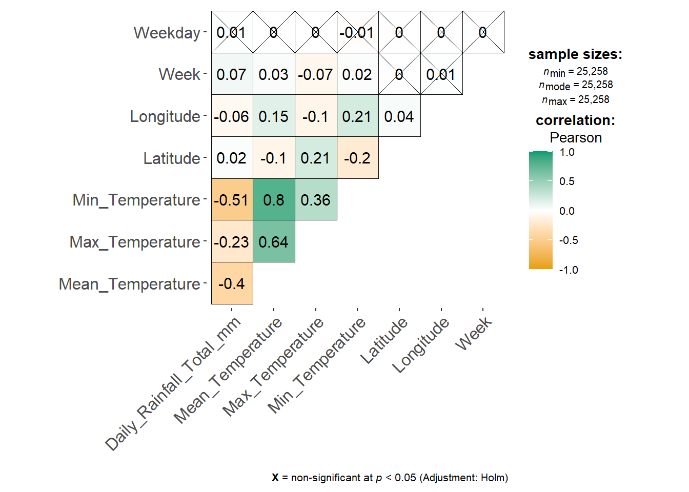
For the explorartory analysis we can use boxplot to see the
data_2023 <- filter(weather_data_imputed, Year == 2023)

# Create the ggplot object
p1 <- ggplot(data = data_2023 %>% filter(Station == "Changi"),
             aes(y = Mean_Temperature, x = Month_Name)) +
  geom_boxplot() +
  theme(axis.text.x = element_text(angle = 45, vjust = 1, hjust=1)) +
  labs(title = "Mean Temperature by Month for Changi Station, 2023",
       y = "Mean Temperature (°C)", x = "Month")

# Convert to an interactive plotly object
p1_interactive <- ggplotly(p1, tooltip = c("y", "x"))

# Display the interactive plot
p1_interactiveggplot(data=weather_data_imputed, aes(x=Date,y=Mean_Temperature)) +
geom_line() + xlab("Year") + ylab("Daily Mean Temperature")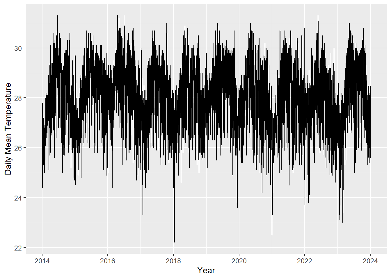
From the time series analysis on top, we clearly see that there is seasonal trend in different months in Singapore.
weather_data_filtered <- weather_data_imputed %>%
  filter(Station == "Changi")  # Filter the data for JFK airport

# Plotting using ggplot2
p <- ggplot(data = weather_data_filtered, aes(x = Date, y = Mean_Temperature, text = paste("Date: ", Date, "<br>Mean Temperature: ", Mean_Temperature))) +
  geom_point() +  # Scatter plot
  xlab("Date") + ylab("Daily Mean Temperature") +
  ggtitle("Mean Temperature at Changi Weather Station")  # Add title

# Convert ggplot to plotly
ggplotly(p)
Horizon Plot:
To have a more clear view of the distribution across the months, we can use a horizon plot to see the distribution and cut points.
# Ensure data has Year, Month, Date column + Date_mine column
weather_data <- weather_data_imputed %>%
  mutate(Year = year(Date)) %>%
  mutate(Month = month(Date)) %>%
  mutate(Day = day(Date)) %>%
  mutate(Date_mine = make_date(2023, month(Date), day(Date)))


# compute origin and  horizon scale cutpoints:
cutoffs <- weather_data %>%
  mutate(
    outlier = between(
      `Mean_Temperature`,
      quantile(`Mean_Temperature`, 0.25, na.rm = TRUE) -
        1.5 * IQR(`Mean_Temperature`, na.rm = TRUE),
      quantile(`Mean_Temperature`, 0.75, na.rm = TRUE) +
        1.5 * IQR(`Mean_Temperature`, na.rm = TRUE))) %>%
  filter(outlier)

ori <- sum(range(cutoffs$`Mean_Temperature`))/2
sca <- seq(range(cutoffs$`Mean_Temperature`)[1],
           range(cutoffs$`Mean_Temperature`)[2],
           length.out = 7)[-4]

ori <- round(ori, 2) # The origin, rounded to 2 decimal places
sca <- round(sca, 2) # The horizon scale cutpoints

# Plot horizon plot
weather_data %>% ggplot() +
  geom_horizon(aes(x = Date_mine,
                   y = `Mean_Temperature`,
                   fill = after_stat(Cutpoints)),
               origin = ori, horizonscale = sca) +
  scale_fill_hcl(palette = 'RdBu', reverse = T) +
  facet_grid(~Station ~ .) +
  theme_few() +
  theme(
    panel.spacing.y = unit(0, "lines"),
    strip.text.y = element_text(size = 7, angle = 0, hjust = 0),
    axis.text.y = element_blank(),
    axis.title.y = element_blank(),
    axis.ticks.y = element_blank(),
    panel.border = element_blank()
    ) +
  scale_x_date(expand = c(0, 0),
               date_breaks = "1 month",
               date_labels = "%b") +
  xlab('Date') +
  ggtitle('Mean Temperature across Month',
          'By different stations')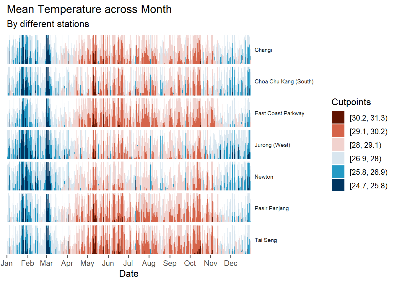
From the Analysis, we can see that clearly there are months with much lower temperature compare to other months. For example, Jan, Feb, Mar we can observe that they mostly have maximum temperature of 28 degrees celcirse
After the data preparation, for exploratory data analysis will be introducing the horizon plot, and tmap to explore the data set will visual.
Boxplot:
box_plot_t1 <- ggplot(weather_data_imputed,
                   aes(y= Mean_Temperature,
                       x = Year)) +
  geom_boxplot()+
  facet_wrap(~Station) +
  theme(axis.text.x = element_text(angle = 60)) +
  scale_x_discrete(name = "Year") +
  scale_y_continuous(name = "Mean Temperature")

box_plot_t1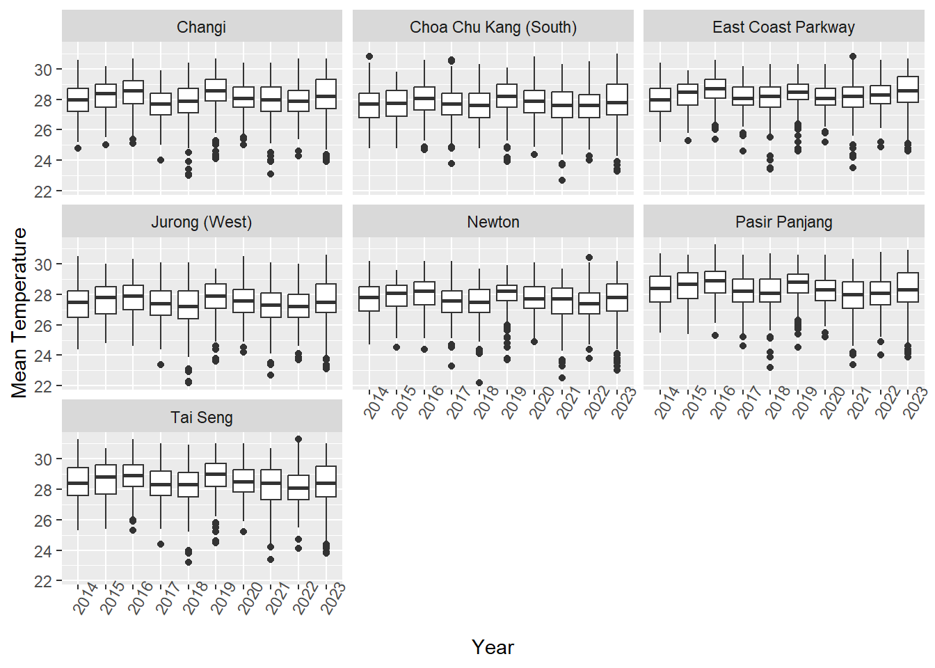
5.2 CDA Hypothesis
This confirmatory data analysis section will check the data based on the certain hypothesis made from the exploratory & descriptive analysis in the above sections.
As of now, two hypothesis are made:
Does Singapore’s weather change across different years shows statistical significant?
can we clearly identify the ‘dry’ and ‘wet’ month?
5.2.1Does Singapore’s Weather Change Across Different Years Shows Statistical Significant?
In this part, the weather change accounts for both the temperature and the rainfall as given in the data used.
5.2.1.1 Temperature
temp_year1 <- weather_data_imputed %>%
  group_by(Station,Year) %>%
  summarise(median_mean_temp = median(Mean_Temperature),
            median_max_temp = median(Max_Temperature),
            median_min_temp = median(Min_Temperature))

DT::datatable(temp_year1,class = "compact")glimpse(temp_year1)Rows: 70
Columns: 5
Groups: Station [7]
$ Station <chr> "Changi", "Changi", "Changi", "Changi", "Changi", "Ch…
$ Year <fct> 2014, 2015, 2016, 2017, 2018, 2019, 2020, 2021, 2022,…
$ median_mean_temp <dbl> 28.00, 28.40, 28.60, 27.70, 27.90, 28.60, 28.10, 28.0…
$ median_max_temp <dbl> 31.9, 32.0, 32.1, 31.3, 31.9, 32.6, 31.9, 32.1, 31.8,…
$ median_min_temp <dbl> 25.20, 25.80, 25.90, 25.10, 25.40, 26.00, 25.40, 25.2…Save the output as csv:
write_csv(temp_year1, "data/temp_year1.csv")To check out the median mean, max and min temperature:
plot_list <- lapply(unique(temp_year1$Station), function(stn) {
  station_data <- subset(temp_year1, Station == stn)

  plot_ly(data = station_data, x = ~Year, y = ~median_mean_temp, name = stn, type = 'scatter', mode = 'lines',
          hoverinfo = 'text', text = ~paste("Station:", stn, "<br>Year:", Year, "<br>Temp:", median_mean_temp)) %>%
    layout(title = paste("Median Mean Temperature - Station:", stn),
           xaxis = list(title = "Year"),
           yaxis = list(title = "Temperature (°C)"))
})

p2 <- subplot(plot_list, nrows = length(unique(temp_year1$Station)), shareX = TRUE, titleX = FALSE)

p2 <- layout(p2,
                       title = "Median Daily Mean Temperature Across Weather Stations (2014-2023)",
                       xaxis = list(tickangle = 90),
                       margin = list(b = 80)) # Increase bottom margin to accommodate angled x-axis labels
p2
Based on the line graph, we can not say that there the mean temperature across selected weather stations have significant changes from year 2014 to 2023.
plot_list <- lapply(unique(temp_year1$Station), function(stn) {
  station_data <- subset(temp_year1, Station == stn)

  plot_ly(data = station_data, x = ~Year, y = ~median_max_temp, name = stn, type = 'scatter', mode = 'lines',
          hoverinfo = 'text', text = ~paste("Station:", stn, "<br>Year:", Year, "<br>Temp:", median_max_temp)) %>%
    layout(title = paste("Median Max Temperature - Station:", stn),
           xaxis = list(title = "Year"),
           yaxis = list(title = "Temperature (°C)"))
})

p3 <- subplot(plot_list, nrows = length(unique(temp_year1$Station)), shareX = TRUE, titleX = FALSE)

p3 <- layout(p3,
                       title = "Median Daily Maximum Temperature Across Weather Stations (2014-2023)",
                       xaxis = list(tickangle = 90),
                       margin = list(b = 80)) # Increase bottom margin to accommodate angled x-axis labels
p3
p4 <- lapply(unique(temp_year1$Station), function(stn) {
station_data <- subset(temp_year1, Station == stn)
plot_ly(data = station_data, x = ~Year, y = ~median_min_temp, name = stn, type = 'scatter', mode = 'lines',
hoverinfo = 'text', text = ~paste("Station:", stn, "<br>Year:", Year, "<br>Temp:", median_min_temp)) %>%
layout(title = paste("Median Min Temperature - Station:", stn),
xaxis = list(title = "Year"),
yaxis = list(title = "Temperature (°C)"))
})
p4 <- subplot(p4, nrows = length(unique(temp_year1$Station)), shareX = TRUE, titleX = FALSE)
p4 <- layout(p4,
title = "Median Daily Minimum Temperature Across Weather Stations (2014-2023)",
xaxis = list(tickangle = 90),
margin = list(b = 80)) # Increase bottom margin to accommodate angled x-axis labels
p4Before performing statistical test on the significant level, is best to determine how the temperature data is distributed in the data. We can observe the normality of the data using ridgeline plots, using the code chunk below:
p5 <- ggplot(weather_data_imputed,
       aes(x = Mean_Temperature,
           y = as.factor(Year),
           fill = 0.5 - abs(0.5 - ..ecdf..))) +
  stat_density_ridges(geom = "density_ridges_gradient",
                      calc_ecdf = TRUE) +
  scale_fill_viridis_c(name = "Tail probability",
                       direction = -1,
                       option="turbo") +
  facet_wrap(~Station, scales = "free_y") +
  theme_ridges(font_size = 12) + # Adjusted for smaller text
  coord_cartesian(xlim = c(0,50)) +
  labs(title="Distribution of Mean Temperature from 2014 to 2023",
       y="Station",
       x="Mean Temperature (°C)")

p5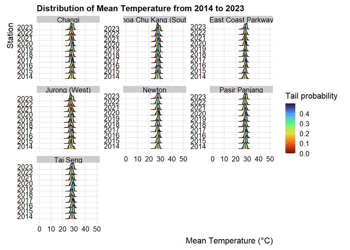
Based on the above observation, as the mean temperature is not normally distributed, non-parametric test will be used.
p6 <- ggplot(weather_data_imputed,
       aes(x = Max_Temperature,
           y = as.factor(Year),
           fill = 0.5 - abs(0.5 - ..ecdf..))) +
  stat_density_ridges(geom = "density_ridges_gradient",
                      calc_ecdf = TRUE) +
  scale_fill_viridis_c(name = "Tail probability",
                       direction = -1,
                       option="turbo")+
  facet_wrap(~Station, scales = "free_y") +
  theme_ridges(font_size = 12)+
  coord_cartesian(xlim = c(0,50))+
  labs(title="Distribution of Maximum Temperature from 2014 to 2023",
       y="Station",
       x="Maximum Temperature (°C)")

p6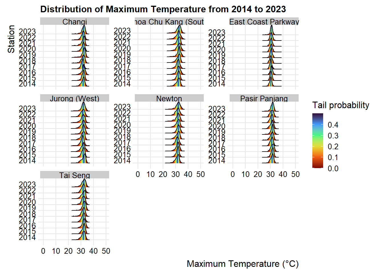
Based on the above observation, as the maximum temperature is not normally distributed, non-parametric test will be used.
p8 <- ggplot(weather_data_imputed,
       aes(x = Min_Temperature,
           y = as.factor(Year),
           fill = 0.5 - abs(0.5 - ..ecdf..))) +
  stat_density_ridges(geom = "density_ridges_gradient",
                      calc_ecdf = TRUE) +
  scale_fill_viridis_c(name = "Tail probability",
                       direction = -1,
                       option="turbo")+
  facet_wrap(~Station, scales = "free_y") +
  theme_ridges(font_size = 12)+
  coord_cartesian(xlim = c(0,50))+
  labs(title="Distribution of Minimum Temperature from 2014 to 2023",
       y="Station",
       x="Minimum Temperature (°C)")

p8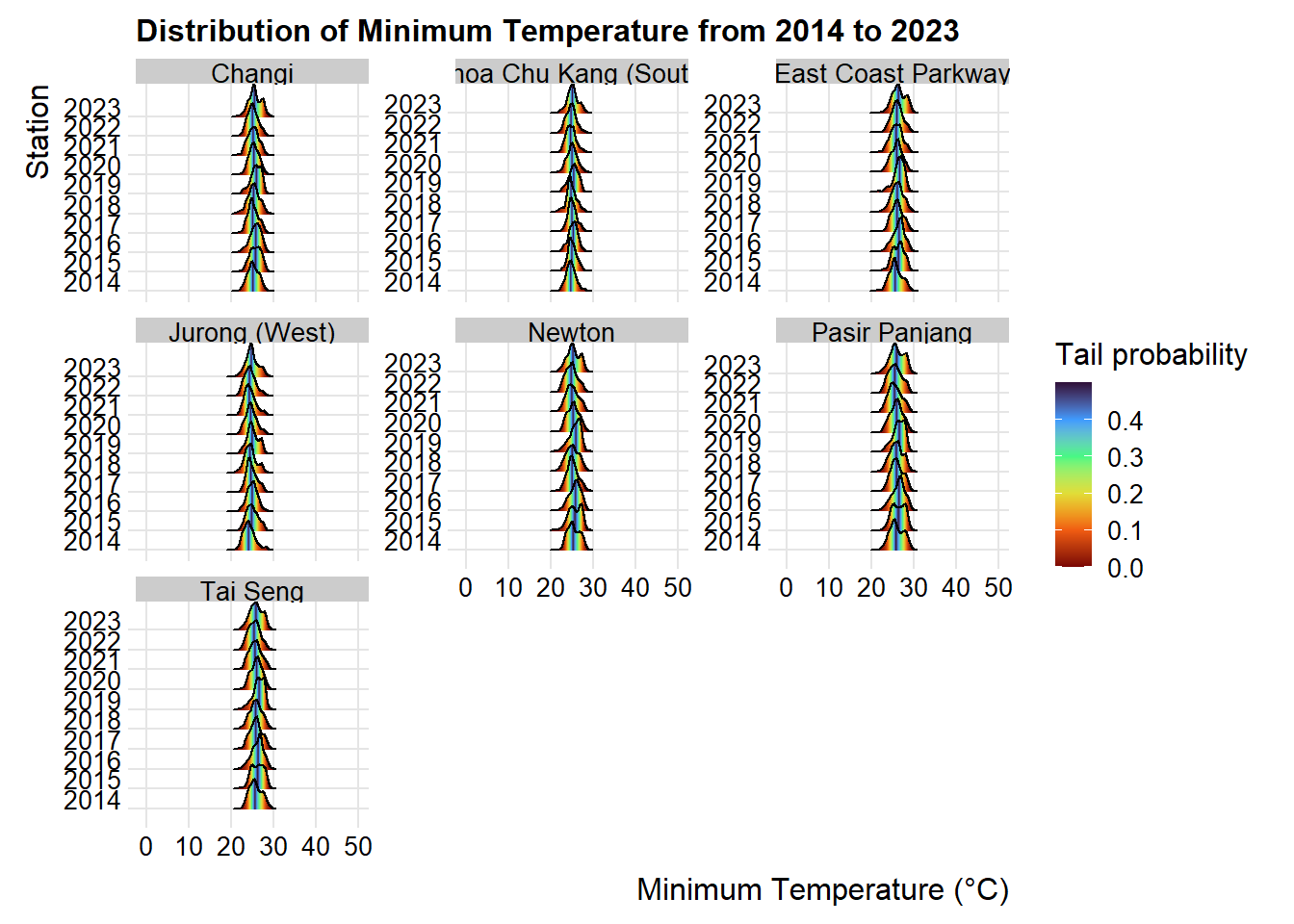
Based on the above observation, as the minimum temperature is not normally distributed, non-parametric test will be used.
Default Non-Parametric tests temperature different per year:
The hypothesis is as follows:
H0: There is no statistical difference between yearly median mean temperature from 2014-2023.
H1: There is statistical difference between yearly median mean temperature from 2014-2023.
p9 <- ggbetweenstats(
  data = temp_year1,
  x = Year,
  y = median_mean_temp,
  type = "np",
  messages = FALSE,
  title="Distribution of Yearly Median Mean Temperature from 2014 to 2023",
  ylab = "Temperature (°C)",
  xlab = "Year",
  ggsignif.args = list(textsize = 4)
) +
  theme(text = element_text(size = 12),plot.title=element_text(size=12))
p9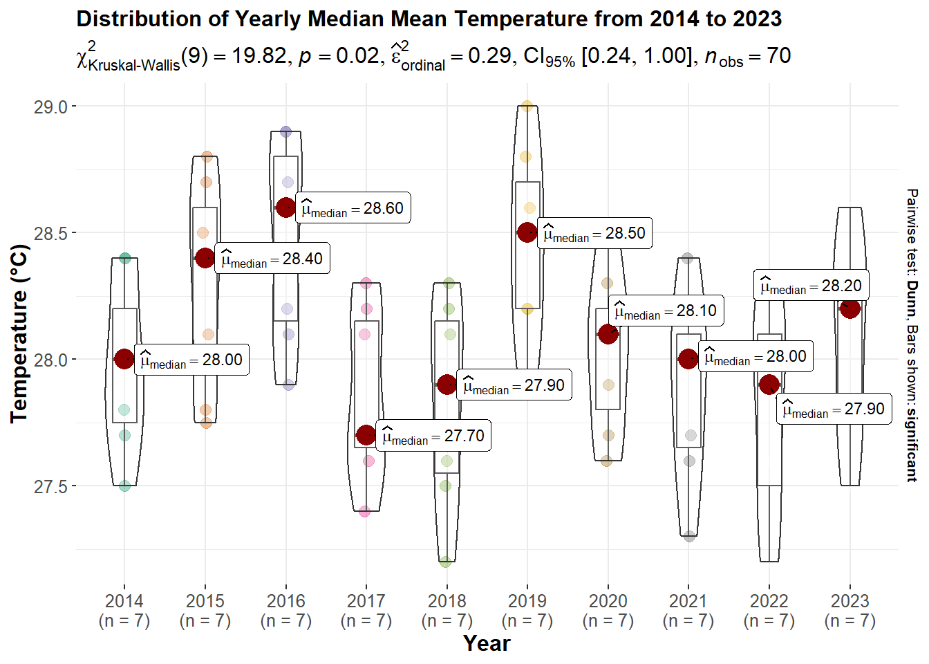
Kruskal-Wallis Test: The test has a x^2 value of 19.82 and a p-value of 0.02, which is below the conventional alpha level of 0.05. This suggests that there is statistically significant difference in median maximum temperatures across the years.
The hypothesis is as follows:
H0: There is no statistical difference between yearly median max temperature from 2014-2023.
H1: There is statistical difference between yearly median max temperature from 2014-2023.
p10 <- ggbetweenstats(
  data = temp_year1,
  x = Year,
  y = median_max_temp,
  type = "np",
  messages = FALSE,
  title="Distribution of Yearly Median Maximum Temperature from 2014 to 2023",
  ylab = "Temperature (°C)",
  xlab = "Year",
  ggsignif.args = list(textsize = 4)
) +
  theme(text = element_text(size = 12),plot.title=element_text(size=12))
p10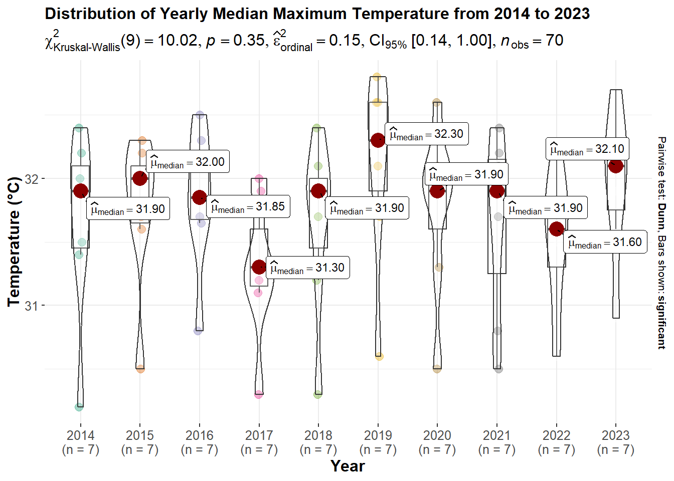
Kruskal-Wallis Test: The test has a x^2 value of 10.02 and a p-value of 0.35, which is above the conventional alpha level of 0.05. This suggests that there is no statistically significant difference in median maximum temperatures across the years. But from yearly difference we can further dig into the daily difference to see if there is a statistical difference.
The hypothesis is as follows:
H0: There is no statistical difference between yearly median min temperature from 2014-2023.
H1: There is statistical difference between yearly median min temperature from 2014-2023.
p11 <- ggbetweenstats(
  data = temp_year1,
  x = Year,
  y = median_min_temp,
  type = "np",
  messages = FALSE,
  title="Distribution of Yearly Median Minimum Temperature from 2014 to 2023",
  ylab = "Temperature (°C)",
  xlab = "Year",
  ggsignif.args = list(textsize = 4)
) +
  theme(text = element_text(size = 12),plot.title=element_text(size=12))
p11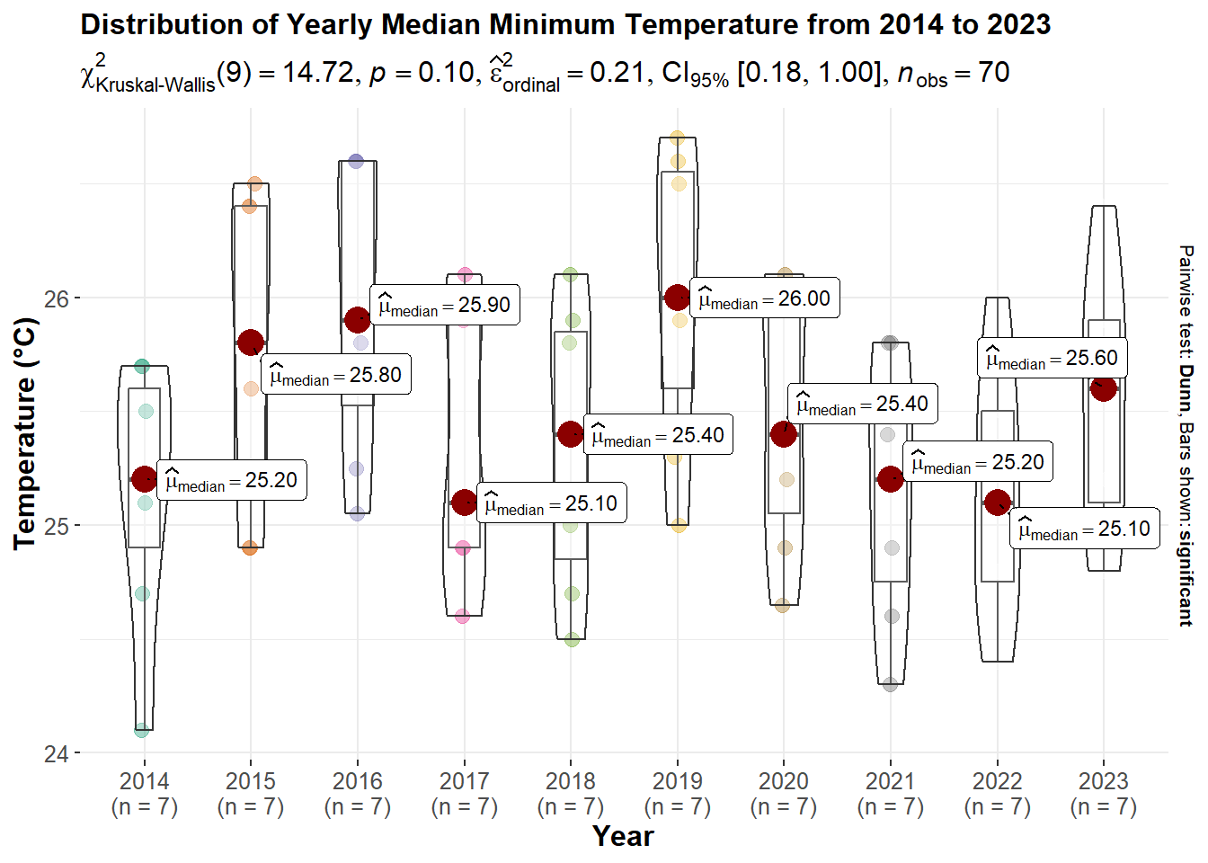
Kruskal-Wallis Test: The test has a x^2 value of 14.72 and a p-value of 0.10, which is above the conventional alpha level of 0.05. This suggests that there is no statistically significant difference in median maximum temperatures across the years. But from yearly difference we can further dig into the daily difference to see if there is a statistical difference.
Hypothesis :
H0: There is no statistical difference in daily mean temperature from 2014-2023.
H1: There is statistical difference in daily mean temperature from 2014-2023.
p12 <- ggbetweenstats(
  data = weather_data_imputed,
  x = Year,
  y = Mean_Temperature,
  type = "np",
  messages = FALSE,
  title="Distribution of Daily Minimum Temperature from 2014 to 2023",
  ylab = "Temperature (°C)",
  xlab = "Year",
  ggsignif.args = list(textsize = 4)
) +
  theme(text = element_text(size = 12),plot.title=element_text(size=12))
p12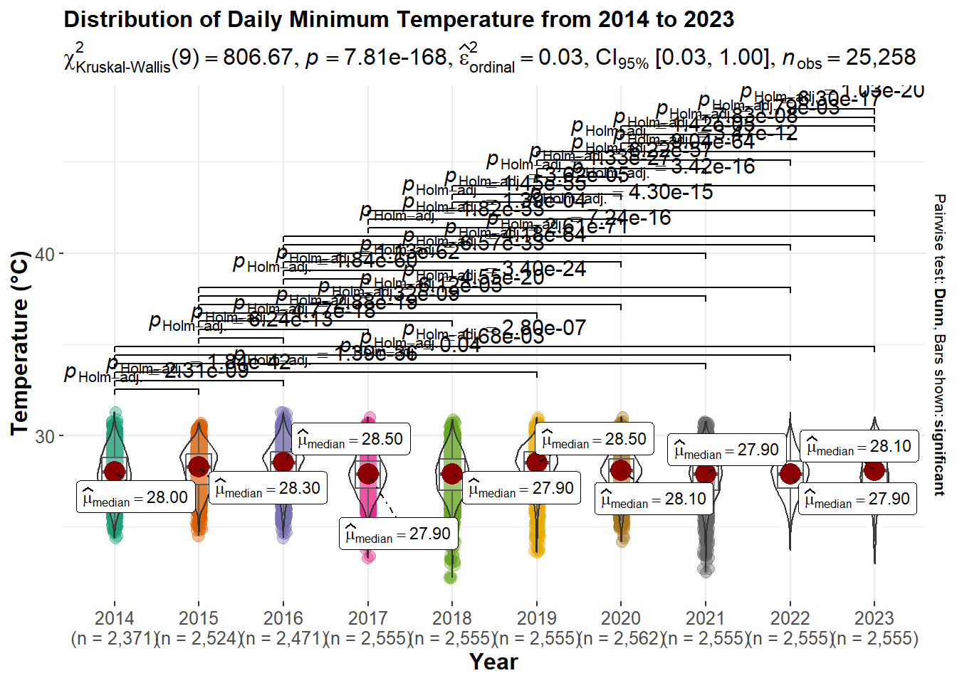
Hypothesis :
H0: There is no statistical difference in daily max temperature from 2014-2023.
H1: There is statistical difference in daily max temperature from 2014-2023.
p13 <- ggbetweenstats(
  data = weather_data_imputed,
  x = Year,
  y = Max_Temperature,
  type = "np",
  messages = FALSE,
  title="Distribution of Daily Maximum Temperature from 2014 to 2023",
  ylab = "Temperature (°C)",
  xlab = "Year",
  ggsignif.args = list(textsize = 4)
) +
  theme(text = element_text(size = 12),plot.title=element_text(size=12))
p13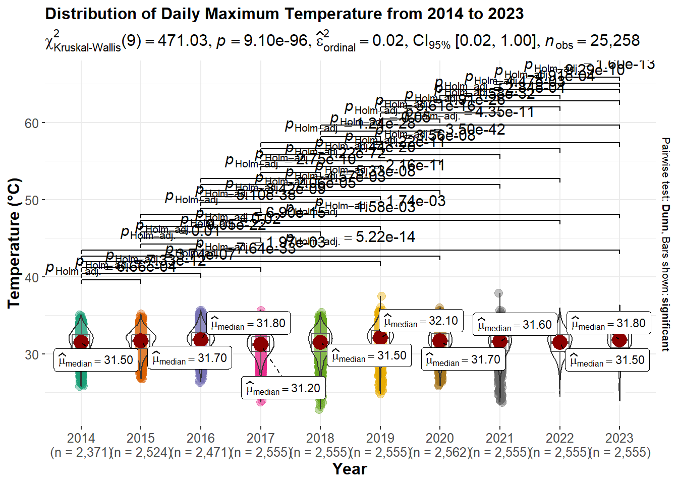
Hypothesis :
H0: There is no statistical difference in daily min temperature from 2014-2023.
H1: There is statistical difference in daily min temperature from 2014-2023.
p14 <- ggbetweenstats(
  data = weather_data_imputed,
  x = Year,
  y = Min_Temperature,
  type = "np",
  messages = FALSE,
  title="Distribution of Daily Minimum Temperature from 2014 to 2023",
  ylab = "Temperature (°C)",
  xlab = "Year",
  ggsignif.args = list(textsize = 4)
) +
  theme(text = element_text(size = 12),plot.title=element_text(size=12))
p14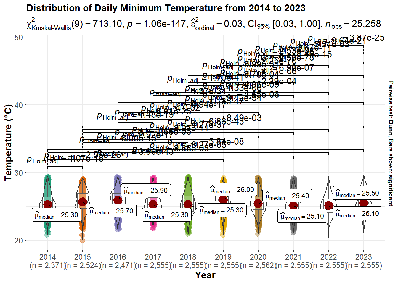
Important
All daily temperatures (mean, maximum and minimum) have p-value lower than 0.05 which means they all shows statistical significant. Meaning there are statistical different in the mean, maximum and minimum daily temperature in Singapore.
- Even though the yearly median max temperature and median min temperature appears no statistical significant, but the daily max and min are statistically different.
5.2.1.2 Rainfall
For rainfall we will be using the daily rainfall total to test the hypothesis
rainfall_year <- weather_data_imputed %>%
  group_by(Station,Year) %>%
  summarise(yearly_rainfall = sum(Daily_Rainfall_Total_mm))

DT::datatable(rainfall_year,class = "compact")write_csv(rainfall_year, "data/rainfall_year.csv")plot_list <- lapply(unique(rainfall_year$Station), function(stn) {
station_data <- subset(rainfall_year, Station == stn)
plot_ly(data = station_data, x = ~Year, y = ~yearly_rainfall, name = stn, type = 'scatter', mode = 'lines') %>%
layout(title = paste("Yearly Rainfall - Station:", stn),
xaxis = list(title = "Year", tickangle = 90),
yaxis = list(title = "Rainfall Volume (mm)"))
})
faceted_plot <- subplot(plot_list, nrows = length(unique(rainfall_year$Station)), shareX = TRUE, titleX = FALSE)
faceted_plot <- layout(faceted_plot,
title = "Yearly Rainfall Across Weather Stations (2014-2023)")
faceted_plotFrom the observations above, over the pass 10 years from 2014 to 2023 the total rainfall for Singapore captured by different stations indicates there is a volume increase. And every a few years it tend to drop to a low point(2015 and 2019) and will bounce back with even higher volume.
We have to check if the different in years of the total rainfall are statistically different, before making any conclusions. But first lets see if the data follows a normal distribution or not in determine the method for test later.
p7 <- ggplot(weather_data_imputed,
       aes(x = Daily_Rainfall_Total_mm,
           y = as.factor(Year),
           fill = 0.5 - abs(0.5 - ..ecdf..))) +
  stat_density_ridges(geom = "density_ridges_gradient",
                      calc_ecdf = TRUE) +
  scale_fill_viridis_c(name = "Tail probability",
                       direction = -1,
                       option="turbo")+
  facet_wrap(~Station) +
  theme_ridges(font_size = 12)+
  coord_cartesian(xlim = c(0,50))+
  labs(title="Distribution of Daily Rainfall from 2014 to 2023",
       y="Station",
       x="Rainfall Volume (mm)")

p7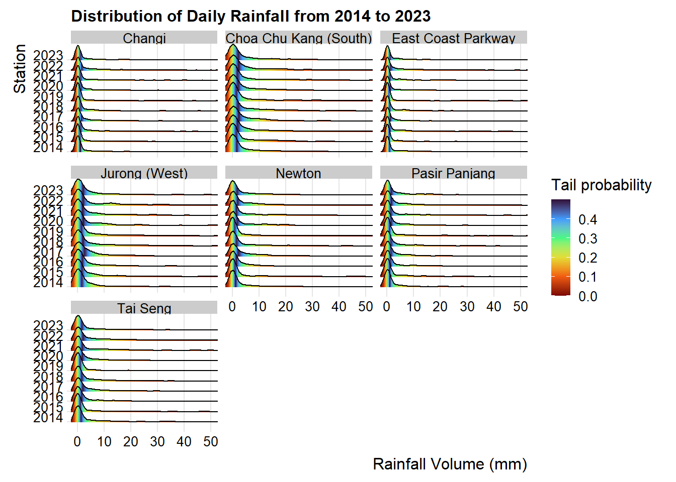
From the distribution graph using sstat function called stat_density_ridges()of ggplot2. We can see that the rainfall distribution is not normally distributed, so non-parametric test will be used.
Hypothesis:
H0: There is no statistical difference between median rainfall per year from 2014-2023.
H1: There is statistical difference between median rainfall per year across 2014-2023.
p8 <- ggbetweenstats(
  data = rainfall_year,
  x = Year,
  y = yearly_rainfall,
  type = "np",
  pairwise.display = "non-significant",
  messages = FALSE,
  title="Distribution of Rainfall from 2014 to 2023",
  ylab = "Rainfall volume (mm)",
  xlab = "Year",
  ggsignif.args = list(textsize = 4)
) +
  theme(text = element_text(size = 12), plot.title=element_text(size=12))

p8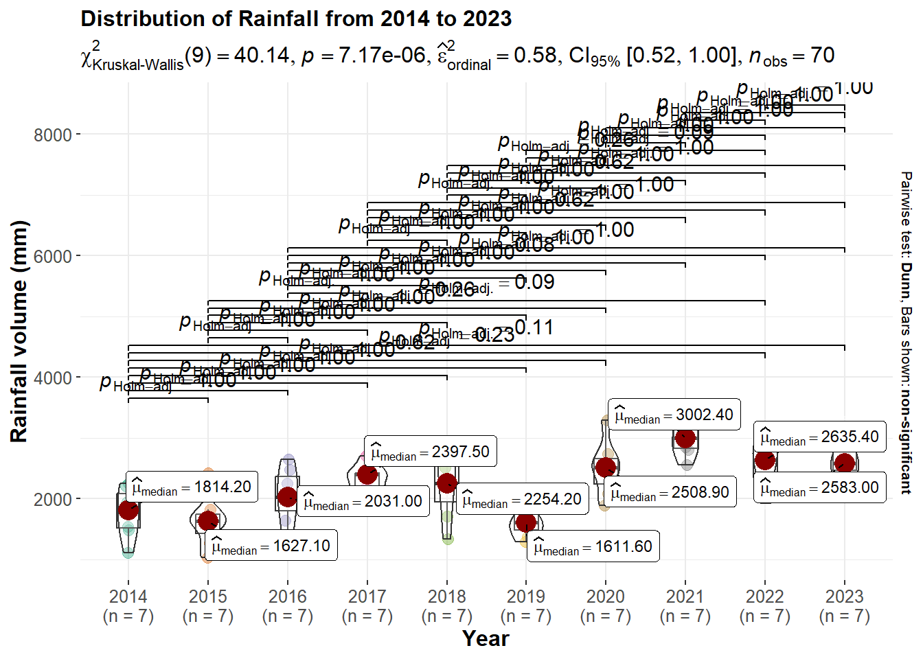
# Filter the data for a specific year
rainfall_year_filtered <- rainfall_year %>%
  filter(Year >= 2014, Year <= 2023)

# Create the plotly violin plot
p8_plotly <- plot_ly(data = rainfall_year_filtered,
                     x = ~Year,
                     y = ~yearly_rainfall,
                     type = 'violin',
                     spanmode = 'hard',
                     marker = list(opacity = 0.5, line = list(width = 2)),
                     box = list(visible = T),
                     points = 'all',
                     scalemode = 'count',
                     meanline = list(visible = T, color = "red"),
                     color = I('#caced8'),
                     marker = list(line = list(width = 2, color = '#caced8'))
                    ) %>%
  layout(title = "Distribution of Rainfall from 2014 to 2023",
         yaxis = list(title = "Rainfall volume (mm)"),
         xaxis = list(title = "Year"))

# Show the plot
p8_plotly
Kruskal-Wallis test result at the top indicates a significant difference in rainfall distribution across the years (p-value < 0.01), suggesting that at least one year has a statistically different total rainfall volume compared to the others.
from the lines connecting the years we can observe that some years trend towards significance when the pHolm-adj is less than 1.00. Hence we can reject the null hypothesis and say that the rainfall over the years is statistically significant.
Hypothesis:
H0: There is no statistical difference between median daily rainfall from 2014-2023.
H1: There is statistical difference between median daily rainfall from 2014-2023.
p9 <- ggbetweenstats(
  data = weather_data_imputed,
  x = Year,
  y = Daily_Rainfall_Total_mm,
  type = "np",
  pairwise.display = "non-significant",
  messages = FALSE,
  title="Distribution of Rainfall from 2014 to 2023",
  ylab = "Rainfall volume (mm)",
  xlab = "Year",
  ggsignif.args = list(textsize = 4)
) +
  theme(text = element_text(size = 12), plot.title=element_text(size=12))

p9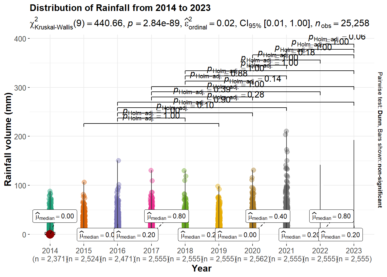
We can dig further into the daily rainfall total to see if there is statistical significant. After undergo the test above, we can observe the test result that overall Kruskal-Wallis test is highly significant (p=2.84e−89), indicating there are differences in the distributions of daily rainfall volumes across the years.
We can also observe that some years the median daily rainfall is 0.00 or 0.20 (2014, 2015, 2019, etc.) suggesting low rainfall volume.
5.2.2 Can We Clearly Identify the ‘Dry’ and ‘Wet’ Month?
Singapore which is a tropical country, means have no clear identification of the four seasons, but there are certain months which the ‘cooler’ compare to some months. In this section we will be testing the hypothesis on ‘can we clearly identify the ’Dry’ and ‘Wet’ Month’?
First we need to filter the data to get monthly records, code chunk below:
rf_data_month <- weather_data_imputed %>%
  group_by(Year,Month) %>%
  summarise(monthly_rainfall = sum(Daily_Rainfall_Total_mm))

rf_data_month$Year <- factor(rf_data_month$Year)
rf_data_month$Month <- factor(rf_data_month$Month, levels = as.character(1:12))

DT::datatable(rf_data_month,class = "compact")glimpse(rf_data_month)Rows: 120
Columns: 3
Groups: Year [10]
$ Year <fct> 2014, 2014, 2014, 2014, 2014, 2014, 2014, 2014, 2014,…
$ Month <fct> 1, 2, 3, 4, 5, 6, 7, 8, 9, 10, 11, 12, 1, 2, 3, 4, 5,…
$ monthly_rainfall <dbl> 450.6, 124.0, 728.1, 1296.2, 1621.8, 1026.9, 1070.8, …temp_month <- weather_data_imputed %>%
group_by(Year,Month) %>%
summarise(median_mean_temp = median(Mean_Temperature),
median_max_temp = median(Max_Temperature),
median_min_temp = median(Min_Temperature))
DT::datatable(temp_month,class = "compact")To see the distribution of the monthly rainfall and Temperature, code chunk below:
color_palette <- brewer.pal("Set3", n = length(unique(rf_data_month$Year)))

p18 <- ggplot(rf_data_month, aes(x = Month, y = monthly_rainfall, fill = Year)) +
  geom_bar(stat = "identity") +
  facet_wrap(~Year, scales = "free_x") +
  labs(title = "Monthly Rainfall From Year 2014 to 2023",
       y = "Rainfall volume (mm)",
       x = "Month") +
  theme_minimal() +
  scale_fill_manual(values = color_palette) +
  theme(panel.spacing.y = unit(0.5, "lines")) # Adjusted for less spacing

p18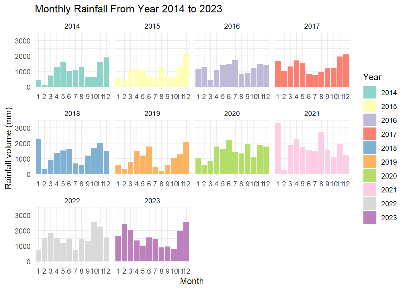
From the distribution of monthly rainfall from year 2014 to 2023, we can observe that the data is not normally distributed, hence non-parametric test will be used later.
p19 <- ggplot(temp_month,
       aes(y = median_mean_temp,
           x = Month,
           colour = Year)) +
  geom_line(size = 1.5)+
  facet_wrap(~Year, scales = "free_x") +
  labs(title="Monthly mean Temperature From 2014 to 2023",
       y = "Temperature (°C)",
       x = "Month")+
  coord_cartesian(ylim = c(20,35))+
  scale_x_discrete(limits = 1:12) + # Assuming Month is numeric already
  theme_minimal() +
  theme(panel.spacing.y = unit(0.5,"lines"))

p19
From the distribution of monthly mean temperature from year 2014 to 2023, we can observe that the data is not normally distributed, hence non-parametric test will be used later.
p20 <- ggplot(temp_month,
       aes(y = median_max_temp,
           x = Month,
           colour = Year)) +
  geom_line(size = 1.5)+
  facet_wrap(~Year, scales = "free_x") +
  labs(title="Monthly Maximum Temperature From 2014 to 2023",
       y = "Temperature (°C)",
       x = "Month")+
  coord_cartesian(ylim = c(20,35))+
  scale_x_discrete(limits = 1:12) + # Assuming Month is numeric already
  theme_minimal() +
  theme(panel.spacing.y = unit(0.5,"lines"))

p20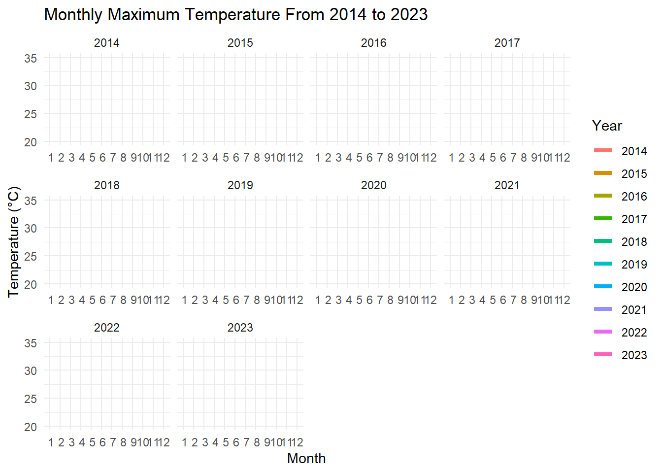
From the distribution of monthly maximum temperature from year 2014 to 2023, we can observe that the data is not normally distributed, hence non-parametric test will be used later.
p21 <- ggplot(temp_month,
       aes(y = median_min_temp,
           x = Month,
           colour = Year)) +
  geom_line(size = 1.5)+
  facet_wrap(~Year, scales = "free_x") +
  labs(title="Monthly Minimum Temperature From 2014 to 2023",
       y = "Temperature (°C)",
       x = "Month")+
  coord_cartesian(ylim = c(20,35))+
  scale_x_discrete(limits = 1:12) + # Assuming Month is numeric already
  theme_minimal() +
  theme(panel.spacing.y = unit(0.5,"lines"))

p21
From the distribution of monthly minimum temperature from year 2014 to 2023, we can observe that the data is not normally distributed, hence non-parametric test will be used later.
5.2.2.1 Hypothesis testing
To test Monthly Rainfall From Year 2014 to 2023:
The hypothesis is as follows:
H0: There is no statistical difference between minimum temperature across months.
H1: There is statistical difference between minimum temperature across months.
Hypothesis:
H0: There is no statistical difference in rainfall volume across months.
H1: There is statistical difference in rainfall volume across months.
p22 <- ggbetweenstats(
  data = rf_data_month,
  x = Month,
  y = monthly_rainfall,
  type = "np",
  messages = FALSE,
  title="Distribution of Rainfall across months 2014 to 2023",
  ylab = "Rainfall volume (mm)",
  xlab = "Month",
  ggsignif.args = list(textsize = 4)
) +
  theme(text = element_text(size = 12), plot.title=element_text(size=12))
p22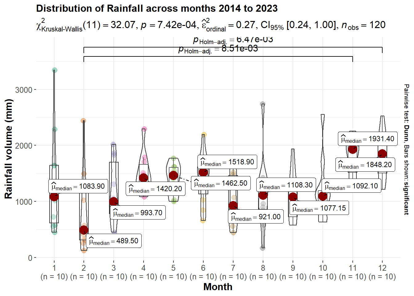
At CI of 95%, the Kruskal-Wallis test results give a p-value < 0.05, which indicates there is statistical difference in the rainfall volume across different month in Singapore.
Feb has significant different in rainfall volume comparing with Nov and Dec.
2, 3, 7, 8, 9, 10 can consider ‘Dry’ as median rainfall volume lower or equal to around 1000mm per month.
4, 5, 6, 11, 12 can consider a ‘Wet’ as median rainfall volume mainly higher than 1400mm per month.
Hypothesis:
H0: There is no statistical difference between mean temperature across months.
H1: There is statistical difference between mean temperature across months.
p23 <- ggbetweenstats(data = temp_month,
                      x = Month,
                      y = median_mean_temp,
                      type = "np",
                      messages = FALSE,
                      title = "Distribution of Mean Temperature by month from 2014 to 2023",
                      ylab = "Temperature (C)",
                      xlab = "Month",
                      ggsignif.args = list(textsize =4)) +
  theme(text = element_text(size = 11),plot.title = element_text(size = 11))
p23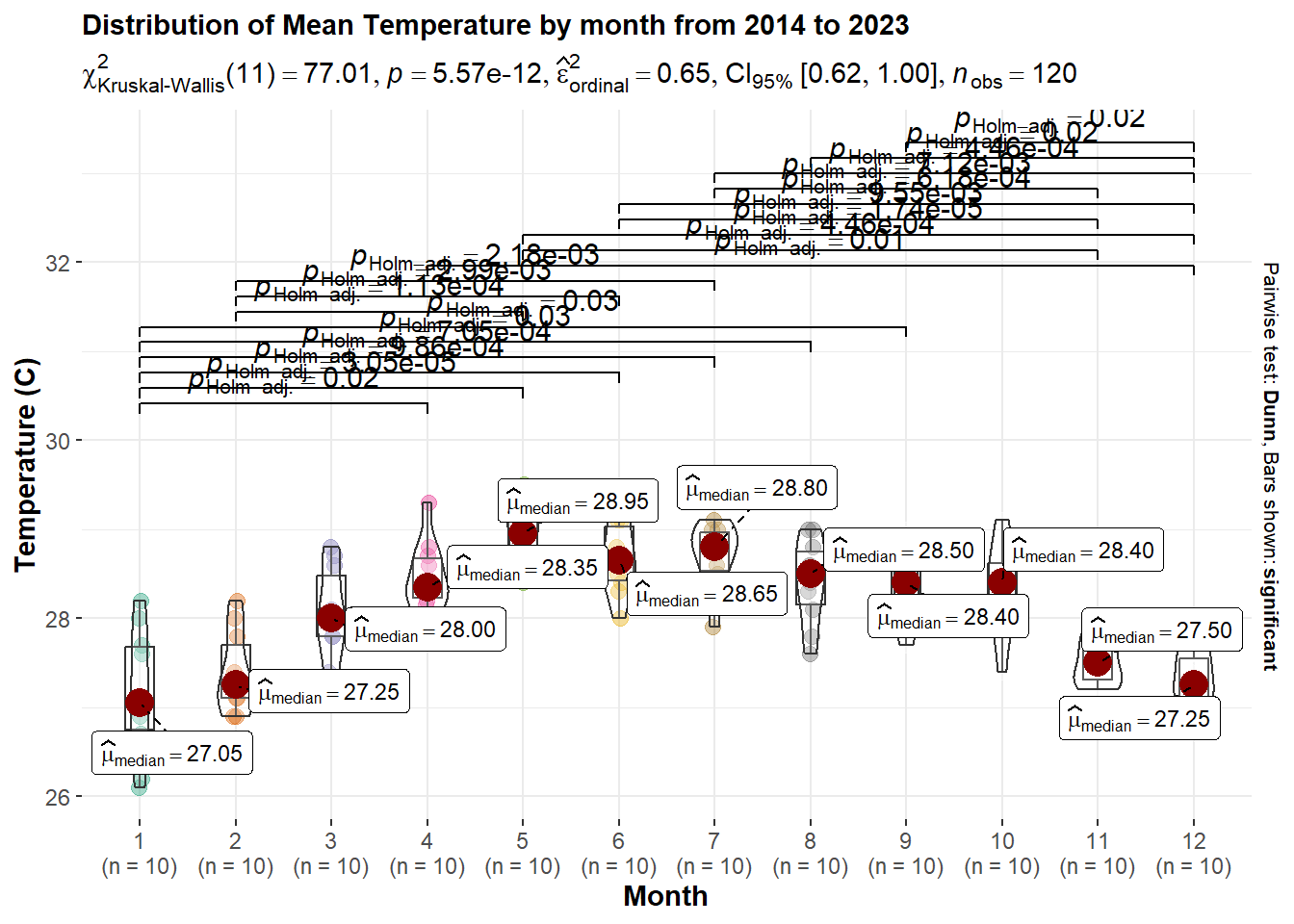
At CI of 95%, the Kruskal-Wallis test results give a p-value < 0.05, which indicates there is statistical difference in the mean temperature across different month in Singapore.
It is observed that towards the middle of the 12 months, 5, 6, 7 ,8 ,9 has the highest median mean temperature .
While months 1, 2, 11, 12 has the lowest median mean temperature.
Hypothesis:
H0: There is no statistical difference between maximum temperature across months.
H1: There is statistical difference between maximum temperature across months.
p24 <- ggbetweenstats(data = temp_month,
                      x = Month,
                      y = median_max_temp,
                      type = "np",
                      messages = FALSE,
                      title = "Distribution of Maximum Temperature by month from 2014 to 2023",
                      ylab = "Temperature (C)",
                      xlab = "Month",
                      ggsignif.args = list(textsize =4)) +
  theme(text = element_text(size = 11),plot.title = element_text(size = 11))
p24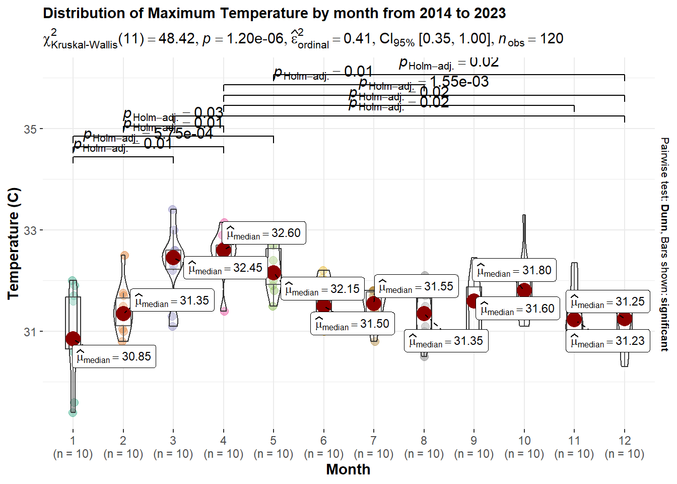
At CI of 95%, the Kruskal-Wallis test results give a p-value < 0.05, which indicates there is statistical difference in the maximum temperature across different month in Singapore.
The month with highest daily temperature is month 3, 4, 5 which average maximum temperature more than 32 Degree Celsius.
Month with lowest daily temperature is January, with only average maximum temperature of 30.85 Degree Celsius.
Hypothesis:
H0: There is no statistical difference between minimum temperature across months.
H1: There is statistical difference between minimum temperature across months.
p25 <- ggbetweenstats(data = temp_month,
                      x = Month,
                      y = median_min_temp,
                      type = "np",
                      messages = FALSE,
                      title = "Distribution of Minimum Temperature by month from 2014 to 2023",
                      ylab = "Temperature (C)",
                      xlab = "Month",
                      ggsignif.args = list(textsize =4)) +
  theme(text = element_text(size = 11),plot.title = element_text(size = 11))
p25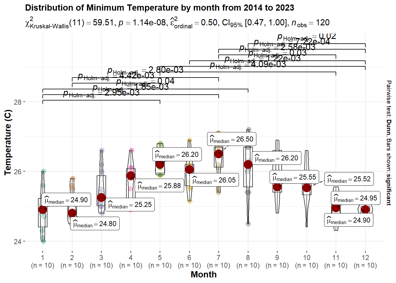
At CI of 95%, the Kruskal-Wallis test results give a p-value < 0.05, which indicates there is statistical difference in the minimum temperature across different month in Singapore.
From the hypothesis testing, result indicates that we can clearly identify the ‘Dry’ or ‘Wet’ months, and also the ‘Hot’ and ‘Cool’ months from the date used.
From the hypothesis testing, several result can be shown:
Dry Month: 2, 3, 7, 8, 9
Wet Month :1, 6, 11, 12
Hot Month: 3, 4, 5, 9, 10
Cool Month: 1, 2, 11, 12
Dry & Hot : 3, 9
Wet & Cool : 1, 11, 12
By identifying this can help Singapore Government to develop strategies to deal with different situations, and also to see the trend in future if there is shift in different type of month
7. UI Design & Layout For Shiny-app
Example for the control pannel there should be check box that affecting the model, not just displaying the changes, Just a sample for EDA:

User also able to select the type of test:
parametric
non-parametric
robust
bayes factor
The plot type to enable user to select among the three options of plot type available for statistical analysis using ggbetweenstats function:
boxplot
violin
violin-boxplot
User able to select the confidence level for the test:
95% CI
99% CI
Pairwise Display:
Significant
Non-significant